What I want to do
I bought a handful of DHT11 sensors. Before putting them in different locations to measure statistically significant differences between the locations, it is important to ensure the sensors have comparable performance.
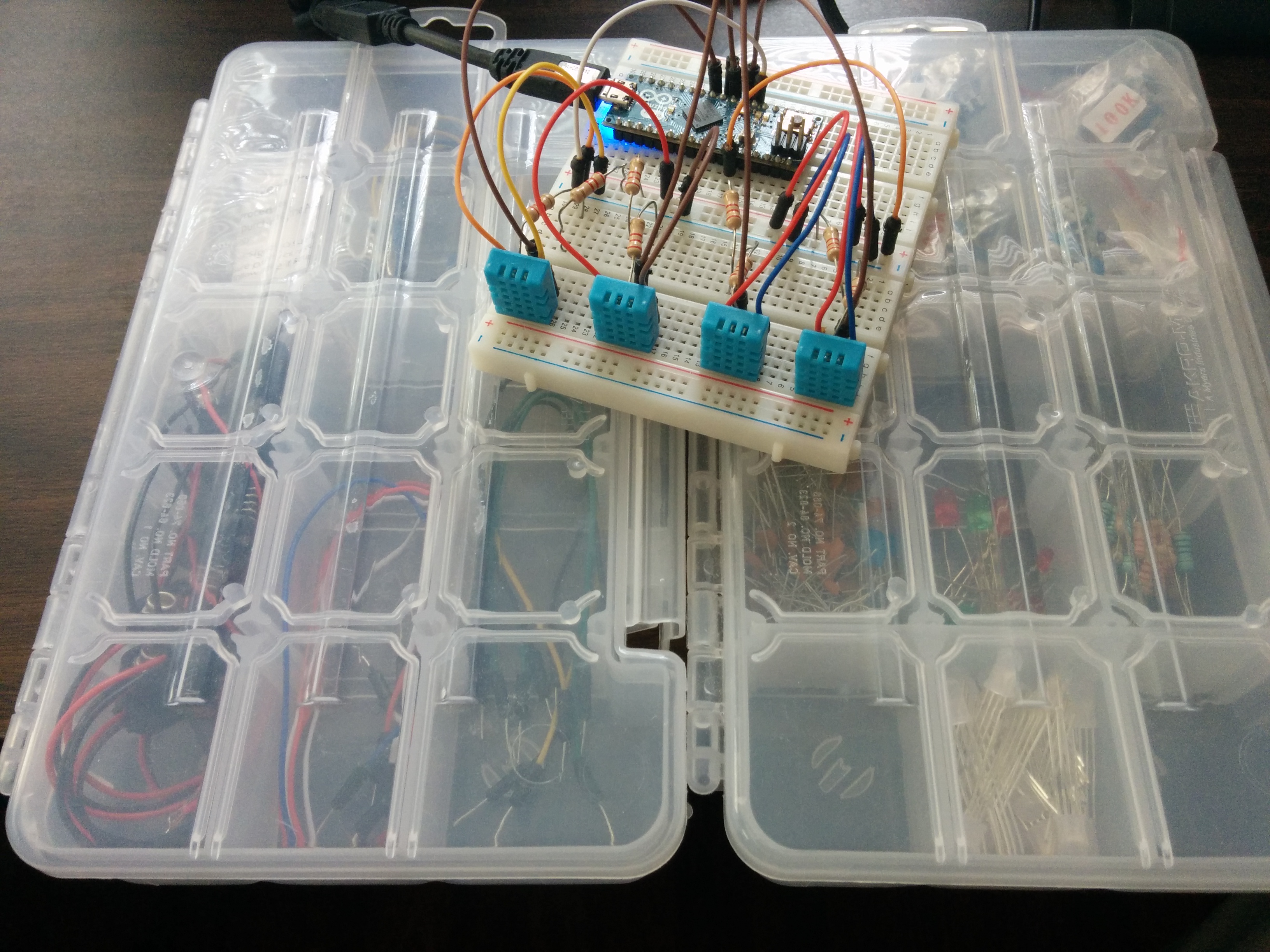
My attempt
I bought four DHT11 sensors from Amazon for less than $2/ea. http://www.amazon.com/gp/product/B007YE0SB6
I grabbed a library from AdaFruit. https://github.com/adafruit/DHT-sensor-library
I installed all four sensors together, physically co-located, so that they should measure the same temperature and relative humidity. I'm using an Arduino Micro (based on the Leonardo architecture) to collect data. The schematics recommended 10k pullup resistors. I was using 2.2k pullup resistors initially, but bumped up to 4.4k pullup resistors (two 2.2k in series). You use what you got, and I got 2.2k ohm resistors. A lot of them.

I wrote some code to collect data from each sensor in a loop and print the data as a CSV to the serial console. No sensor should be polled more than once every 2 seconds according to AdaFruit's writeup of the sensors. There are no useful timestamps in Arduino, so each loop will increment a cycle counter. The cycle counter will be modified to represent a timestamp (no doubt with some error) later on.
 #include <stdio.h>
 #include "DHT.h"

 DHT* dht;
 const int nSensors = 4;
 int cycle;

 void setup() {
   Serial.begin(9600);
   Serial.println("Serial initialized...");

   dht = (DHT*)malloc(nSensors*sizeof(DHT));
   for (int i=0; i<nSensors; i++) {
     // assumes first sensor is pin 2 and
     // each subsequent sensor is plugged into the next pin down
     dht[i] = DHT(i+2, DHT11);
     dht[i].begin();
   }

   cycle=0;
 }

 void loop() {
   char buffer[64];
   for (int i=0; i<nSensors; i++) {
     // iterate the entire set of sensors in approximately 2 seconds, with a little buffer.
     delay(2000./nSensors + 250);
     float h = dht[i].readHumidity();
     float t = dht[i].readTemperature();
     if (isnan(h) || isnan(t)) {
       Serial.println("No good boss.");
       continue;
     }
     // print CSV with cycle number, sensor number, humidity (in %), and temp (in Celsius).
     sprintf(buffer,"%6d,%d,%2d,%2d",cycle,i,int(h),int(t));
     Serial.println(buffer);
   }
   cycle++;
 }
Install pyserial for a convenient interface to serial devices. Actually I use
miniterm.pydirectly.miniterm.py /dev/ttyACM0 | tee 201407140130.csvCollect data over a long period of time. I started mine in my bedroom at 1:30am local time. I turned off my AC unit and opened the room to the outdoors at about noon local time. I planned to end data collection at 1:30pm local time, but I must have disconnected the Arduino by accident around 12:47pm. I timestamped the start of the data collection into the filename (see above), and then included the end time in the filename at the end (see below). The start and end times will be used to determine the cycle-to-timestamp conversion.
mv 201407140130.csv 201407140130t2014071247.csvClean data. Once data collection was complete, I parsed the beginning and end of the csv. The first cycle (cycle 0) only had data from two sensors because the command wasn't run early enough (it will be impractical to line this up perfectly anyway). So I deleted the partial cycle 0 from the data. Similarly the last cycle (cycle 9839) only had two sensors of data, so it was also deleted.
Import csv to numpy. I wrote a quick script for this.
 import csv
 import numpy

 if __name__ == "__main__":
   import sys
   if len(sys.argv) != 2:
     print "Run {0} <filename>".format(sys.argv[0])
     sys.exit(1)
   filename=sys.argv[1]

   print "Opening file {0} and converting to numpy array".format(filename)
   with open(filename, 'r') as csvfile:
     reader = csv.reader(csvfile)
     # build initial array
     array = numpy.array([reader.next()], dtype=int)
     # iterate through rows, expanding the array.
     for row in reader:
       array = numpy.concatenate((array, numpy.array([row], dtype=int)))

   print "Writing out array to file."
   filenameout = filename + ".npy"
   with open(filenameout, 'w') as arrayfile:
     numpy.save(arrayfile, array)

   print "Done."
Normalize the data. The RH and temp across each sensor should be independently converted to normal form for later analysis.
 >>> import numpy
 >>> # get data
 >>> data = numpy.load('201407140134t201407141247.csv.npy')
 >>> norm = data.astype('double')
 >>> for i in range(0,4):
 ...   selection = data[:,1] == i
 ...   for j in range(2,4):
 ...     chunk = norm[selection,j]
 ...     norm[selection,j] = (chunk - numpy.mean(chunk))/numpy.std(chunk)
 ...
 >>> norm.save('DHT11normalized.npy')

My results
Timing
I measured the cycle times to be approximately 4 seconds per cycle, when they were intended to be 2 seconds. I added an arbitrary 250ms to each sensor as a buffer, but I should have added 250ms/N. Since there are 4 sensors, that arbitrary buffer adds a total of 1 second to the entire cycle. The cycle itself ignoring the arbitrary delay and processing time, should be 2s long. So that's a total of 3s cycles ignoring data processing time. It looks like data processing per cycle is surprisingly on the order of 250ms per sensor (1s to the total cycle time). I flubbed those calculations but it isn't a big deal.
I determined the conversion from cycle to timestamp by assuming a uniform distribution of cycles from the beginning time to the end time. This is a linear fit of the form y = mx + b. The slope m was found to be about 4 seconds per cycle. For the first cycle in the csv, x = 1 and y(1) = 2014-07-14 1:34am. b was found to be a time just before 1:34am. A double check for the last cycle's time shows that it begins one cycle-time prior to the end time, which is what we want. Python datetime and timedelta objects are nice, but b really should be UTC time since epoch; that is shown as utcb below. So given any cycle number x, the UTC time since epoch in seconds y can be found with y = 4.104910*x + 1405316035.8955088. Use that formula to replace cycle number with timestamp in place.
    >>> import numpy
    >>> # get data
    >>> data = numpy.load('201407140134t201407141247.csv.npy')
    >>> import datetime
    >>> # establish time frame
    >>> begin = datetime.datetime(2014,7,14,1,34)
    >>> end = datetime.datetime(2014,7,14,12,47)
    >>> # look at start and end cycle numbers
    >>> data[0]
    array([ 1,  0, 39, 27])
    >>> data[-1]
    array([9838,    3,   43,   31])
    >>> # find time elapsed per cycle
    >>> m = (end - begin) / int(data[-1][0] - data[0][0])
    >>> m
    datetime.timedelta(0, 4, 104910)
    >>> # find y-intercept given x=1
    >>> b=begin-m
    >>> b
    datetime.datetime(2014, 7, 14, 1, 33, 55, 895090)
    >>> #confirm end times match
    >>> b + m*int(data[-1][0])
    datetime.datetime(2014, 7, 14, 12, 46, 55, 887804)
    >>> end
    datetime.datetime(2014, 7, 14, 12, 47)
    >>> # convert b from UTC-0400 to UTC epoch.
    >>> utcb = (b + datetime.timedelta(hours=4) - datetime.datetime.utcfromtimestamp(0)).total_seconds()
    >>> utcb
    1405316035.8955088
    >>> # replace cycle number with timestamps
    >>> data[:,0] = data[:,0]*m.total_seconds() + utcb
    >>> # save modified data
    >>> data.save('DHT11colocate.npy')
Visual Inspection
It is always good to visually inspect the data. Here are two graphs, one for temperature and one for RH, and the code used to generate them. They appear to track each other well over time, with a possible +/- 2 Celsius degree error on temperature and +/- 3 whole percent error on relative humidity.


    >>> import numpy
    >>> import matplotlib
    >>> xfmt = matplotlib.dates.DateFormatter('%H:%M:%S')
    >>> arr = numpy.load('DHT11colocate.npy')
    >>> for i in range(0,4):
    ...   selection = arr[:,1] == i
    ...   # change 3 to 2 for RH
    ...   pyplot.plot(matplotlib.dates.epoch2num(arr[selection, 0]), arr[selection, 3])
    ...
    [<matplotlib.lines.Line2D object at 0x2ef7f10>]
    [<matplotlib.lines.Line2D object at 0x2ef7990>]
    [<matplotlib.lines.Line2D object at 0x2ef7650>]
    [<matplotlib.lines.Line2D object at 0x2f11510>]
    >>> pyplot.gca().xaxis.set_major_formatter(xfmt)
    >>> pyplot.xlabel("Time")
    <matplotlib.text.Text object at 0x37d97d0>
    >>> pyplot.ylabel("Temperature (Celsius)")
    <matplotlib.text.Text object at 0x32e7390>
    >>> pyplot.legend(["Sensor 1", "Sensor 2", "Sensor 3", "Sensor 4"], loc="upper left")
    <matplotlib.legend.Legend object at 0x2ef77d0>
Cross Correlation for Temperature
Cross correlation between sensors can show if there is a time delay between sensors responding to signals and visual inspection can give some sense of how well the pairs of sensors relate to each other.
In the case of temperature, the correlations are quite high (the lowest correlation is 0.91 between sensors 1 and 4). In the zoomed in image, one can see that the peaks all appear at cycle offset 0. This means there does not appear to be any time shift between sensors (not that one was expected). Generally the correlations between sensors track very well for low cycle offsets. The correlation drops off over long periods of time because the data has no strong repetition over time.


In the case of relative humidity, the correlations are still quite high (the lowest correlation is 0.86 between sensors 1 and 2), but not as highly correlated as temperature. In the zoomed image, one can see the peak occurs at cycle offset 0 here as well. The relative humidity measurements show much more cyclic action because the measured relative humidity measured bounced up and down between small values, unlike temperature which remained relatively flat.


    >>> pyplot.plot(numpy.correlate(norm[data[:,1]==0,2], norm[data[:,1]==1,2], "full")/9838)
    [<matplotlib.lines.Line2D object at 0x93213d0>]
    >>> pyplot.plot(numpy.correlate(norm[data[:,1]==0,2], norm[data[:,1]==2,2], "full")/9838)
    [<matplotlib.lines.Line2D object at 0x93219d0>]
    >>> pyplot.plot(numpy.correlate(norm[data[:,1]==0,2], norm[data[:,1]==3,2], "full")/9838)
    [<matplotlib.lines.Line2D object at 0x6815d5d0>]
    >>> pyplot.plot(numpy.correlate(norm[data[:,1]==1,2], norm[data[:,1]==2,2], "full")/9838)
    [<matplotlib.lines.Line2D object at 0x6815d310>]
    >>> pyplot.plot(numpy.correlate(norm[data[:,1]==1,2], norm[data[:,1]==3,2], "full")/9838)
    [<matplotlib.lines.Line2D object at 0x6815df90>]
    >>> pyplot.plot(numpy.correlate(norm[data[:,1]==2,2], norm[data[:,1]==3,2], "full")/9838)
    [<matplotlib.lines.Line2D object at 0x9158cd0>]
    >>> pyplot.xlabel('cycle offset')
    <matplotlib.text.Text object at 0x683349d0>
    >>> pyplot.ylabel('normalized correlation for RH')
    <matplotlib.text.Text object at 0x68172a10>
    >>> pyplot.legend(['1v2', '1v3', '1v4', '2v3', '2v4', '3v4'])
    <matplotlib.legend.Legend object at 0x9158590>
    >>> pyplot.xticks([0, cycles, cycles*2],[-cycles/2, 0, cycles/2])([<matplotlib.axis.XTick object at 0x683341d0>, <matplotlib.axis.XTick object at 0x68334fd0>, <matplotlib.axis.XTick object at 0x6815b250>], <a list of 3 Text xticklabel objects>)
Post-Hoc Hypothesis Testing
Consider the hypothesis that each of these sensors is measuring the same temperature, and a separate hypothesis that each of these sensors is measuring the same RH. This desired hypothesis assumes there is no difference between measurements on the average which is a pretty standard null hypothesis. Unfortunately, one can never really accept the null hypothesis.
Nearly all hypothesis tests desire to show that distributions are different by first assuming they are the same. The mathematics of testing demonstrate a confidence about how badly that assumption was broken. As much as I'd like to drop a confidence interval on how likely these measurements are to be the same, it seems I am unable to find a strategy which is accepted.
Conclusion
Based on visual inspection and cross correlation, I think these sensors are close enough.
Precision
This entire post has been a question of precision: how similar are the measurements to each other. They certainly follow each other well. The good news is that precision is the important characteristic when separating sensors which are meant to be compared against each other. That is precisely what I aim to do. Relative measurements are good enough.
Accuracy
Unfortunately I don't have any gold standard thermometers, thermistors, or other temperature measurement device. I'm pretty certain that these sensors are not accurate, because with my AC running, they were telling me the temperature inside was the same as the temperature outside, which my phone told me through weather services. Accuracy is usually important when working with the NIST or producing devices which are meant to deliver absolute measurements. This is not important to my goal.
Questions and next steps
Why did I add a constant time delta inside an iterative loop without considering the number of sensors? That was silly of me. It should have been more like 2250/n.
The next step is to install these sensors in different locations for a different experiment to see how efficient my AC units are.
Why I'm interested
I used to do sensor data collection in a previous life. Calibration and semi-rigorous testing of the sensors was an important pre-deployment step to ensure valid data is collected. This is a required step before making use of these sensors to see if I should bother running my ACs at certain times of day in the south Florida summer.
4 Comments
Really wonderful writeup. the SHT11, 15, and 21 are all sensors that we're looking to deploy and its good to see an initial look at their precision.
I also want to complement the way you broke down your arduino sketch to highlight what different sections are doing; that is very helpful. really good integration of natural and machine language.
Reply to this comment...
Log in to comment
Thanks mathew. In computer science, it's often taught that programming languages come and go, but clarity is always required. To that end, we would frequently have coding projects where we had to turn in just the comments of what we plan to do without any real code as the first assignment. The next assignment would be to add the code which realizes the comments.
I tend to love comments and readable code for pedagogical reasons and because I'm big into open source. Open source does not work well unless people can pick up the code and just get it.
Reply to this comment...
Log in to comment
i like this elegant strategy!!
Reply to this comment...
Log in to comment
Hello btbonval! Thank you for sharing this project with us! I really liked it. I'm a beginner with Arduino and I would like to make a monitoring to my beehives that shows on a computer graphically. I have a struggle with code writing. Thanks.
Reply to this comment...
Log in to comment
Login to comment.